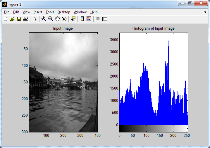
Anyone who has ever used an old television set will likely have encountered salt and pepper noise before. It is sometimes referred to casually as a “fuzzy” or “snowy” screen. Salt and pepper noise is simply the random scattering of black and white pixels throughout an image, which looks like a picture with black and white specs (ie: salt and pepper) all over the image. Consider the sample image and its respective histogram, shown below.

Sample image and histogram

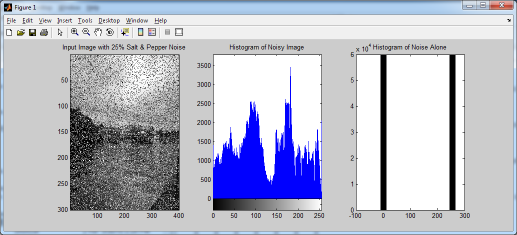
Now, observe the effects randomly making 25% of the pixels in this image either black or white.

Image with noise

Notice the item in the far right of the above image, the spectrum of just the noise: It’s all either black or white. This noise spectrum gives us an idea of how (from a statistics standpoint) salt and pepper noise affects an image. Please note: when I refer to the “noise spectrum”, simply imagine a blank image (ie: every pixel value is zero), and then noise is applied to it.

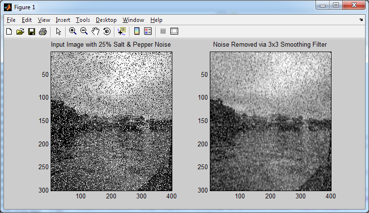
So, now that we have a rough idea of what this kind of noise is, we need to figure out how to deal with it. One simple approach would be to apply a smoothing/blurring filter, which is covered in the previous section on convolution masks. Let’s try this out, and see what happens.

Salt and pepper noise removal attempted via blurring

Well, the results above are less than encouraging. The output image almost looks worse. Since blurring effectively calculates an output pixel’s value based on the values of the neighboring pixels in the source image, salt and pepper noise will not be affected much, if at all, by this filtering method. From a statistics standpoint, the introduction of extreme outliers into a data set will significantly affect the average/mean value of the data set.

What we need is an approach that considers the neighboring pixels in the source image, and ignores outliers. If we think back to simple statistics, one method should stick out above the others: calculating the median. For those who don’t recall what the median is, consider a a set of numbers. Now sort the numbers (ascending or descending, either way works). Now find the value in the exact middle of this sorted list. There is your median value. When introducing extreme values to a data set, the median is rarely affected at all, as the extreme values will remain at either of the two extrema of the sorted data set.

So, let’s try filtering this image again. We will use a median mask, which is a non-linear filter. Think of it like a convolution mask from the previous section, but instead of calculating a sum of products for each overlapping section of the input image and the convolution mask, we will instead calculate the median value. So, for a 3×3 median filter mask, we would have nine (9) pixel values from the source image which we would arrange into a 1-dimensional list, sort numerically, then pick the value in the middle of this list, and assign its value to the appropriate pixel in the output image buffer. A simple recap with respect to convolution masks is shown below.

Median convolution mask equivalent

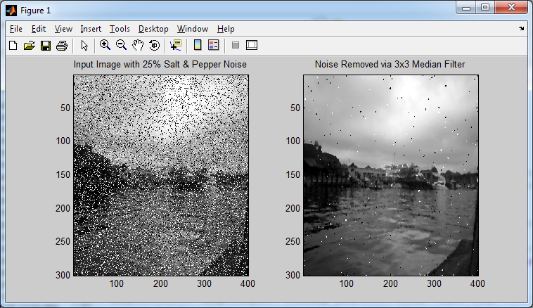
Now, let’s try the median filter on the previous example:

Noise removal of 25% salt and pepper noise via a 3×3 median filter mask

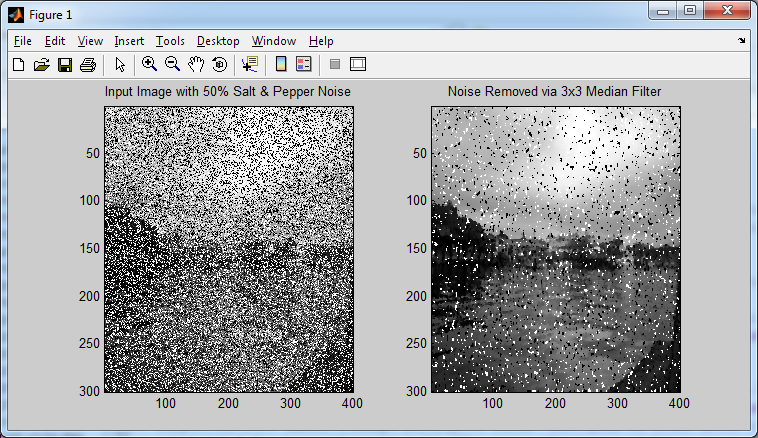
The results are far better than when we attempted noise removal via blurring. Now let’s increase the noise density to 50%.

Noise removal of 50% salt and pepper noise via a 3×3 median filter mask

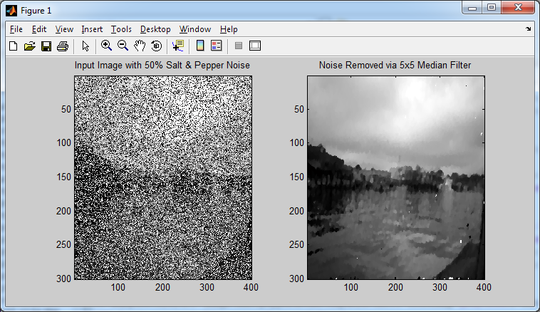
Well, the result isn’t half bad, considering that half of all the pixels in the source image have been randomly been set to a value of black or white. We can still do better though. Let’s increase the size of the median filter mask to 5×5, so that each pixel in the output image is calculated based on 25 pixels from the input image.

Noise removal of 50% salt and pepper noise via a 5×5 median filter mask

Now nearly all of the salt and pepper noise has been removed, but the output image has been distorted considerably. This is an important consideration to take into place when using median filters for this purpose: you will have to find a trade-off between how much noise you want removed, and how much distortion is acceptable in the final result. The functions I wrote to create salt and pepper noise, as well as the median filtering function, are included below. You can use them to apply varying amounts of noise, and to test out median filters of arbitrary sizes (3×3, 5×5, 11×11, etc).

Salt and Pepper Noise Generation:

%==========================================================================
function output_image = saltpeppernoise( input_image, spdensity )
%   output_image    -   The processed image
%   input_image     -   The source image data
%   spdensity       -   The density (ie: percent noise, on [0,1] of salt &
%                       pepper noise
% (C) 2010 Matthew Giassa, <teo@giassa.net> www.giassa.net
%==========================================================================
%Make sure the density is in an allowable range
if((spdensity) <0 || (spdensity>1))
 error('Salt and pepper density level is outside of [0,1]');
end

%Simple definitions
PEPPER_VALUE = double(intmin('uint8'));
SALT_VALUE = double(intmax('uint8'));

%Make a grayscale copy of our input image
I = double(rgb2gray(input_image));

%Determine input image dimensions
[j k] = size(I);

%Determine the total number of pixels
n_pixels = j*k;

%Calculate how many pixels to change
n_noisy_pixels = round(n_pixels * spdensity);

%Determine pixels to modify
%Rows and Columns are essentially row/column indexes that have been sorted
%in a random fashion. If we want to simplify this algorithm even more, an
%alternative approach (ie: in C/C++) would be to create arrays with the
%values 0 through j or k to achieve the same effect
noise_index = randperm(n_pixels);
noise_index = noise_index(1:n_noisy_pixels);

%Since the above index vectors are already randomized, we'll simply assign
%'0' (pepper) values to the first half, and '255' (salt) values to the
%other half. Not the most elaborate method, but works nonetheless
%First, let's reshape the image
I = reshape(I,1,[]);
for counter = 1:n_noisy_pixels./2
 I(noise_index(counter)) = PEPPER_VALUE;
end
for counter = n_noisy_pixels./2+1:n_noisy_pixels
 I(noise_index(counter)) = SALT_VALUE;
end
%Revert the image back from a 1D vector to a 2D image
I = reshape(I,j,k);

output_image = I;

Median Filter:

%==========================================================================
function[A] = imgMaskMed(src_matrix,dim_matrix)
% imgMask   Applies a variable sized median filter to an image
% src_matrix is the original image to copy and modify afterwards
% dim_matrix is the dimension of the mask size

% Copy original image data to a temporary buffer
% and flatten to a 2D grayscale matrix
copy_matrix = src_matrix;

% Determine the dimensions of the source matrix
[x,y] = size(copy_matrix);

% Determine the dimensions to use for the median filter
a = dim_matrix;
b = dim_matrix;

% Error checking code
% Non-square mask matrix
if(a~=b)
 disp(sprintf('Mask matrix is not square!'))
elsif((a==0) | (b==0))
 disp(sprintf('Mask matrix has a singleton dimension!'))
elsif((a<3) | (b<3))
 disp(sprintf('Mask matrix is not at least 3x3!'))
elsif((a>=(x-1)) | (b>=(y-1)))
 disp(sprintf('Mask matrix dimenions are too large!'))
else
 % Pad the matrix edges so we don't lose data
 for j = 1:b
 [a_temp, b_temp] = size(copy_matrix);
 copy_matrix = vertcat(copy_matrix, copy_matrix(a_temp,:));
 copy_matrix = vertcat(copy_matrix(1,:), copy_matrix);
 copy_matrix = horzcat(copy_matrix, copy_matrix(:,b_temp));
 copy_matrix = horzcat(copy_matrix(:,1), copy_matrix);
 end
 % Re-read the new (padded) image size
 [x,y] = size(copy_matrix);
 % Generate a vector containing all elements of the mask matrix
 median_matrix = [];
 for k1=1+ceil(b/2):y-ceil(b/2)
 for k2=1+ceil(a/2):x-ceil(a/2)
 for k3=1:b
 for k4 = 1:a
 median_matrix = horzcat(median_matrix,copy_matrix(k2-floor(b/2)+k4,k1-floor(a/2)+k3));
 end
 end
 copy_matrix(k2,k1) = median(median_matrix);
 median_matrix = [];
 end
 end

 % Trim the matrix edges so input resolution = output resolution
 for j = 1:b
 [a_temp, b_temp] = size(copy_matrix);
 copy_matrix(a_temp,:) = [];
 copy_matrix(:,b_temp) = [];
 copy_matrix(1,:) = [];
 copy_matrix(:,1) = [];
 end
end
%==========================================================================
%======= Complete
%==========================================================================

A = copy_matrix;