Nearest neighbour interpolation is the simplest approach to interpolation. Rather than calculate an average value by some weighting criteria or generate an intermediate value based on complicated rules, this method simply determines the “nearest” neighbouring pixel, and assumes the intensity value of it.

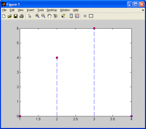
First, let’s consider this in a 1-dimensional case. Observe the plot below.

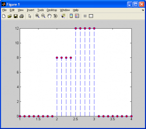
Let’s say that we wanted to insert more data points between the points x1 (=2) and x2 (=3), that approximate the values between them, which range between f(x1) (=4) and f(x2) (=6). Using nearest neighbour interpolation, our result would look like:

We can see above that for each data point, xi, between our original data points, x1 and x2, we assign them a value f(xi) based on which of the original data points was closer along the horizontal axis.

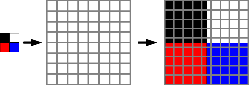
Now, extending this to 2D, assume that we want to re-size a tiny, 2×2 pixel image, X, as shown below, so that it “fits” in the larger 9×9 image grid, Y, to the right of it.

As shown above, when we resize by a non-integral factor (as outlined in the beginnging of this section on interpolation) pixels cannot simply be cloned by column/row – we need to interpolate them. The squares (representing pixels) forming a vertical and horizontal line through the rightmost image, for example, cannot contain different color values. They can only contain a single color value.

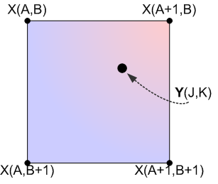
To visualize nearest neighbour interpolation, consider the diagram below. The data points in the set X represent pixels from the original source image, while the data points in the set Y represent pixels in our target output image.

So, for each pixel in the output image Y, we must calculate the nearest neighbouring pixel in our source image X. Furthermore, we should only need to rely on 4 specific data points: X(A,B), X(A+1,B), X(A,B+1), and X(A+1,B+1). We can handle this decision very quickly with a few IF statements, as outlined in the pseudocode below.

START

IF ( K-B < B+1-K)

     Pixel is one of the top two

ELSE

     Pixel is one of the bottom two

ENDIF

IF ( J-A < A+1-J)

     Pixel is one of the "left" two

ELSE

     Pixel is one of the "right" two

ENDIF

DONE

 

This is very straightforward, but how do we properly index our images when we are dealing with an image larger than 2×2 pixels? We need a transformation that will handle this. Consider a small image which is ‘m’ pixels wide by ‘n’ pixels high, which we want to re-size to ‘p’ pixels wide by ‘q’ pixels high, assuming that p>m and q>n. Now, we need two scaling constants:

• s1 = p/m
• s2 = q/n

Now, we simply loop through all the pixels in the target/output image, addressing the source pixels to copy from by scaling our control variables by s1 and s2, and rounding the resulting scaled index values. The following example shows this in action on a 2×2 pixel “checkerboard” pattern image.

%Import my original picture file

I = imread('checker.bmp','bmp');

%Convert image to grayscale (intensity) values for simplicity (for now)

I = rgb2gray(I);

%Determine the dimensions of the source image

%Note that we will have three values - width, height, and the number

%of color vectors, 3

[j k] = size(I);

%Specify the new image dimensions we want for our larger output image

x_new = 640;

y_new = 480;

%Determine the ratio of the old dimensions compared to the new dimensions

%Referred to as S1 and S2 in my tutorial

x_scale = x_new./(j-1);

y_scale = y_new./(k-1);

%Declare and initialize an output image buffer

M = zeros(x_new,y_new);

%Generate the output image

for count1 = 0:x_new-1

 for count2 = 0:y_new-1

 M(count1+1,count2+1) = I(1+round(count1./x_scale),1+round(count2./y_scale));

 end

end

%Display the two images side-by-side for a few seconds, then close

subplot(1,2,1); imagesc(I);colormap gray;

subplot(1,2,2); imagesc(M);colormap gray;

%Write the images to files

imwrite(I,gray(256),'input.jpg');

imwrite(M,gray(256),'output.jpg');

pause(4);

close all;

 

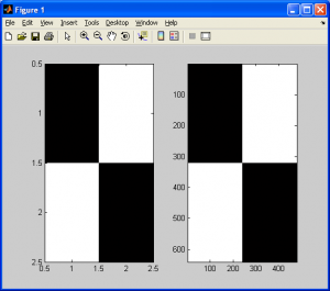
As shown in the images below, the 2×2 checkerboard image was upsampled to a 640×480 pixel image without any changes at all. Furthermore, due to the simplicity of this algorithm, the operation takes very little time to complete. Note the units on the axes for the images below. They look the same, but the one on the left is actually MUCH smaller than the one on the right.

The major drawback to this algorithm is that, despite its speed and simplicity, it tends to generate images of poor quality. Although the checkerboard pattern was upsampled flawlessly, images such as photographs come out “blocky”, though with little to no noticable loss of sharpness, as demonstrated below. The key point here is that this is a simple and fast algorithm. Included below are two more examples that demonstrate the drawbacks of this algorithm.

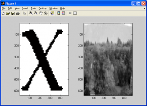
Now, after applying the nearest neighbour algorithm, we get the following results:

As we can see in the results above (you can click on it to get a better view) the results are of poor quality. Although the sharpness of the original image is retained, we notice how the image on the left of an ‘X’ has “jaggies” (ie: jagged edges) and the image on the right looks pixelated and distorted. This is referred to as aliasing, and there are several ways to deal with it. Two of the most straightforward ways are using a better interpolation method, as covered on the proceeding subsection on interpolation, or the use of spatial domain image filtering, which is covered in the sections on filtering. Finally, included below is the code used to generate the above results, along with the nearest neighbour algorithm MATLAB code rewritten as a MATLAB M-function for convenience.

Nearest Neighbour M-Function:

%Nearest neighbour code re-written as a MATLAB function

%==========================================================================

function output_image = nn(input_image,x_res,y_res)

%==========================================================================

%   output_image    :   a grayscale image of dimensions x_res by y_res

%   input_image     :   an arbitray input image with dimensions less than

%                       x_res by y_res

%   x_res           :   the horizontal resolution of the output image

%   y_res           :   the vertical resolution of the output image

%==========================================================================

%Import my original picture file

I = input_image;

%Convert image to grayscale (intensity) values for simplicity (for now)

I = rgb2gray(I);

%Determine the dimensions of the source image

%Note that we will have three values - width, height, and the number

%of color vectors, 3

[j k] = size(I);

%Specify the new image dimensions we want for our larger output image

x_new = x_res;

y_new = y_res;

%Determine the ratio of the old dimensions compared to the new dimensions

%Referred to as S1 and S2 in my tutorial

x_scale = x_new./(j-1);

y_scale = y_new./(k-1);

%Declare and initialize an output image buffer

M = zeros(x_new,y_new);

%Generate the output image

for count1 = 0:x_new-1

 for count2 = 0:y_new-1

 M(count1+1,count2+1) = I(1+round(count1./x_scale),1+round(count2./y_scale));

 end

end

output_image = M;

 

Sample Code:

a1 = imread('x.png','png');

a2 = imread('trees_small.jpg','jpg');

b1 = nn(a1,640,480);

b2 = nn(a2,640,480);

subplot(1,2,1);imagesc(b1);colormap(gray);

subplot(1,2,2);imagesc(b2);colormap(gray);