Before we proceed, I should note that all these tutorials can be used for image processing in general, but the exact code implementations are designed for use with MATLAB R2007 a or later, and the image processing library must be available. For most people this means that unless you shell out some cash for a student version, or you are using lab computers, you will no normally have access to this program. That’s OK though, as the code is generic enough to be ported to C/C++, Java, etc.

So, the first thing we should cover is addressing individual pixels in an image. In MATLAB, once we’ve imported a sample 2D image, we’d like to be able to read and write individual pixels for starters. For those who are already familir with the concept of 2D arrays in a language like C or Java, this should be very straightforward. For a full-color JPEG image such as a digital photograph, each picture element (pixel) can be represented as a three dimensional vector with the following vector components:

• x-coordinate
• y-coordinate
• color-vector

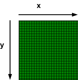
The coordinates should be simple enough to understand as the location of each pixel in an image, as shown below:

But what about the third value, the color-vector? This is a vector itself consisting of 3 color intensity values, one each for:

• Red intensity value
• Blue intensity value
• Green intensity value

So, if you wanted to set a pixel at location (A,B) to black, you would set the RGB (red, green, blue) intensity values all to zero, while if you wanted it to be white, you would set them all to their maximum possible values (changes depending on the image type you are working with; this could be the value 255, 65535, etc). Any other combinations of different intensity values for each of these color values gives you different colors in the discrete color spectrum your software can produce.

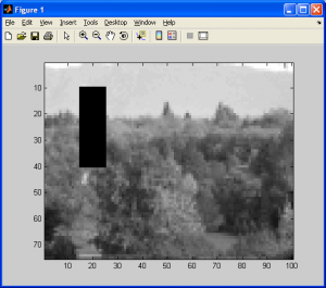
Now that we know this, I’ll let you know right now that most of the tutorials will be working with grayscale images only. Why? Well, for starters, it will make learning this material much easier, and it’s very easy to extend these techniques to color images one you’ve learned them. If I want to import a simple JPEG image, convert it to grayscale, and set some pixels to black, I need to do the following in MATLAB:

a1 = rgb2gray(imread('trees_small.jpg','jpg'));
a1(10:40,15:25) = 0;
imagesc(a1); colormap(gray);

 

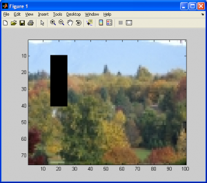
If I want to do the same with a color image, I need to repeat the above code for each of the three color vectors, which would look like:

a1 = imread('trees_small.jpg','jpg');

for counter = 1:3

 a1(10:40,15:25,[counter]) = 0;

end

image(a1);

 

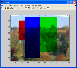
If I want to have some real fun, I could play around with the “counter” control variable so that my loop only cycles through some of the color vectors. You can do this to play with the “tint” (sometimes referred to as colorization) of the image. The following code does just this, as you can see in the following image.

a1 = imread('trees_small.jpg','jpg');

for counter = 2:3

 a1(10:40,15:25,[counter]) = 0;

end

for counter = 1:2

 a1(4:70,26:50,[counter]) = 0;

end

for counter = 1:2:3

 a1(4:60,51:80,[counter]) = 0;

end

image(a1);

 

So, in general, for a simple grayscale image (ie: let’s assume this means 256 shades of gray from white to black), it is easier to address the pixel intensity values rather than having to write code to deal with each of the RGB values. If you want to extend your own code to deal with color images, simply use the “counter” loop as shown in the above code and you’re set! Don’t let this scare you from attempting to design some interesting code that works with color images. I am doing this simply so that it is easier to use these tutorials while avoiding syntax errors that will likely abound if you aren’t yet comfortable with arrays and MATLAB’s array/matrix notation (note that arrays and matrices are NOT the same thing!)

Now, to make things more interesting, I will now import a MAYO 7.5 3D image of a human brain, with dimensions AxBxC (WIDTHxHEIGHTxDEPTH). Note that this 3D image is seen as a 3D array in MATLAB. Note that each array element has a single intensity value (grayscale), and each array element is addressed using 3 coordinates. This can be seen as a 4-dimensional vector (x-y-z coordinates and an intensity value). If this were a color 3D image, it would be a 4-dimensional vector, with the intensity value being replaced by a vector of 3 separate RGB values.

Next, I will take a 2D cross-sectional “slice” of the brain, which can be represented as a 3D, AxBx1 image. With the use of the “squeeze” command in MATLAB, the image is reduced to a proper, 2D, AxB image.

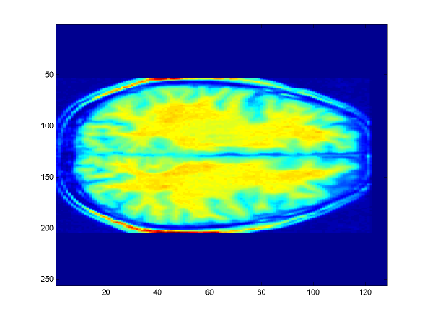
%Import the MAYO 7.5 HDR 3D image of a brain disp(sprintf('Import the MAYO 7.5 HDR 3D image of a brain\n')) I = analyze75read('ibsr_01_ana.hdr'); pause(2) %Determine the height value for where the slice is made disp(sprintf('We will now determine the height of slice\n')) disp(sprintf('A height of 100 elements has been chosen arbitrarily\n')) H = 100; pause(2) %Extract a single 2D slice of the 3D image at height 'H' disp(sprintf('We will now actually extract a slice of the 3D image at the\n')) disp(sprintf('pre-chosen height\n')) J = I(H,:,:); pause(3) %Report the size of J disp(sprintf('The dimensions of the slice are as follows:\n')) size(J) pause(4) %Squeeze the slice dimensions to a MxN matrix %Please note that squeeze effectively copies a matrix, while dropping %any "singleton dimensions" (MATLAB 2007 Help File) disp(sprintf('We will now perform the squeeze() operation on our image slice\n')) disp(sprintf('Basically, it converts the 1xMxN 3D array to a 2D MxN array, since\n')) disp(sprintf('we want a 2D image, and the singleton dimension is extraneous\n')) K = squeeze(J); pause(3) %Report size of squeezed image disp(sprintf('The new dimensions/size of our image are now\n')) size(K) pause(4) %Display the 2D image on-screen disp(sprintf('And here is our image...\n')) imagesc(K) % Save the image to disk for part 2 of the experiment print(['-dbmp'], 'screenshot.bmp');

 

A sample screen shot is shown below, generated using the code shown above.

 

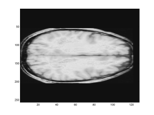
You will notice that the above image is colored quite nicely. This is due to the use of the imagesc command in MATLAB. It takes a grayscale image, and displays it using a colormap of your choosing. This is referred to as false coloring, and can be misleading at times, as the original image was a grayscale one, not a full color image (brains aren’t rainbow colored, in case anyone was wondering). If I want the same image to appear in grayscale, I simply replace the line:

imagesc(K)

With…

imagesc(K); colormap gray;