Ever wondered how to resize an image? Simple – throw away data. When “shrinking” an image’s dimensions (note: this is NOT the same as image compression, which will be covered much later), you are essentially throwing away image information.

Suppose you have an image with dimensions AxB, and you want to shrink it to the dimensions of CxD, assuming that A>C and B>D. The most straightforward way to do this is to discard entire columns/rows of data. How do we know which ones to discard though?

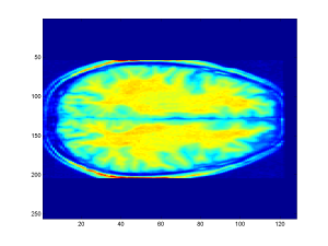
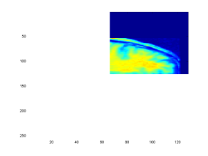
Well, in case you haven’t guessed already, there should be some sort of pattern and reason to this. One naive way is to simply discard pixels at the edges of the image. For the sample image shown below, we delete the first (A-C) columns, and the first (B-D) rows. The result is less than desirable. We’ve effectively cropped out a large portion of the original image.

Standard Image

Cropped Image

So, what approach should we take? Simple! First, calculate the number of columns you will need to discard, k. Since the original number of columns is A, and the new number of columns is C, it only makes sense that we need to discard (A-C) columns. So, assuming we have a sample image, I, and an output image buffer, J, we can create our new, downsampled image in J using the following pseudo-code:

FOR(counter1 = 1 to C) LOOP
J(column(counter1)) = I(column(FLOOR(counter1*A/C)))
END LOOP

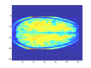
The same code can be changed readily to downsample the rows as well. The columns and rows marked for deletion are represented with white lines, as shown below:

Columns/rows Marked for Deletion

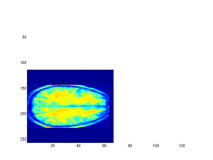
Once we’ve processed/generated the final output image, we get the following:

Downsampled Image

Just to drive the point home, I must again emphasize that image data has been permanently lost, which should make sense, as we’ve deleted entire columns/rows. Taking the downsampled image from above, I have “zoomed in” on it to demonstrate this point, as can be seen by the “blocky” lower-quality image.

Downsampled Image (Zoomed-In)

Finally, included below is a sample application written in MATLAB to demonstrate how to do this kind of operation without relying too much on existing packages and libraries. A final set of sample images are shown side-by-side, demonstrating what happens when we downsample by a large ratio. In the case of the image below, the width was downsampled by a factor of 7, and the height by a factor of 5. Zoomed-in, we can see a considerable loss of quality.

Downsampled Image – Before and After

%Import my original picture file
I = imread('trees.jpg','jpg');
%Convert image to grayscale (intensity) values for simplicity (for now)
I = rgb2gray(I);

%Determine the dimensions of the source image
%Note that we will have three values - width, height, and the number
%of color vectors, 3
[j k] = size(I)

%Specify the new image dimensions we want for our smaller output image
%In this case we will downsample the image by a fixed ratio
%Since the ratios are different, the image will appear distored
%We can also set x_new and y_new to arbitrary values, but it will not work
%if they are larger than j and k. That would be upsampling/interpolation,
%and will be covered in a future tutorial.
x_new = j./7;
y_new = k./5;

%Determine the ratio of the old dimensions compared to the new dimensions
x_scale = j./x_new;
y_scale = k./y_new;

%Declare and initialize an output image buffer
M = zeros(x_new,y_new);

%Generate the output image
for count1 = 1:x_new
 for count2 = 1:y_new
 M(count1,count2) = I(count1.*x_scale,count2.*y_scale);
 end
end

%Display the two images side-by-side for a few seconds, then close
subplot(1,2,1); imagesc(I);colormap gray; axis tight;
subplot(1,2,2); imagesc(M);colormap gray; axis tight;
pause(4);
close all;